Initial Concept Proposal

The Affordable Care Act Mortality Considerations

*NOTE: the project focus has evolved* Read: https://github.com/cbuschnotes/practicum2

High level description of the project: what question or problem are you addressing?

The political climate in the United States is causing turmoil for the Affordable Care Act. One party is trying to actively repeal or destroy it while another party lacks the votes to try to preserve it. In addition, there is a lot of misinformation and confusion around the impacts of the Affordable Care Act health insurance coverage on the residents in the United States. The goal of this study is to detect a mortality improvement “signal” using the CDC mortality public use data files.

The CDC NHIS reports that the level of uninsured has nearly been cut in half (Clarke, Norris, & Schiller, 2017).

<image to go here>

Due to the ACA law, more people are insured so when disease strikes more can seek appropriate care. For example, a Duke University School of Medicine study showed that the rates of cancer patients receiving radiation dropped in half during the first year of Medicaid expansion for the States that adopted it (Knopf, 2017).

Khanna (2017) writes that for the states in which Medicaid expansion did not occur, there is disproportional effect and which uninsured rates for minority patients did not improve while white patients had an improvement in the rate of being insured. It is presumed that improvement resulted from the ACA exchanges.

It may stand to reason that benefits for those with cancer which resulted from coverage may also apply to other diseases as well. However, there is much debate.

<image to go here>

Prior Research and Ongoing Debate


A 2012 study reported in the New England Journal of Medicine found that states in which Medicaid expansions took place a significant reduction in all-cause mortality occurred down about 19.6 death per 100,000 adults (Sommers, Baicker, & Epstein, 2012).

However, conservatives write that mortality has increased or stayed the same. For example, Frankie (2017) writes in the Federalist promoting those concerns.

Unfortunately, there is a study to back up that assessment. Baicker, et al. (2013) found that “Medicaid coverage generated no significant improvements in measured physical health outcomes in the first 2 years”. The authors of that study did note an increase use of Health Care Services and detection rates as well as reduced financial strain. One could easily argue that is not an actual health outcome difference but rather a financial difference.


Hypothesis


Decreasing the uninsured rate has a significant lowering impact on mortality rates when adjusted for an aging population.

The above may be too broad. Possible narrowing of the hypothesis could be:

  • focus on infant mortality
  • focus preventable and manageable diseases.

Potentially Preventable and Manageable Diseases

COPD

Bacterial Pneumonia

Diabetic Ketoacidosis

Hypertension


Presentation

How do you plan to present your work? (visualization or demo, etc.)

The intent is to publish a blog post that includes visualizations. The idea being the visualizations offer compelling evidence that increased Health Care coverage helps to prevent mortality.

Method

How will you analyze the data? What machine learning methods do you plan to use?

First the data will be gathered. ICD 10 codes will be analyzed as markers for diseases types. Regression analysis and feature selection will look for confounding reasons for mortality differences. Age differences will be factored out through resampling techniques or through weighted regression.


Data

Data: Brief description of data. How big do you expect the data will be? Is amount of your data too big or too small? If you’re web-scraping or collecting data, how long do you expect to collect the data?

CDC, County Health Rankings & Roadmaps, and US Census information will be utilized.

The CDC offers a query tool (WONDER) in which raw data can be retrieved for further analysis. In addition, the CDC offers public use files of mortality records. The public use files are about 83 megabytes per year. As mentioned in the Debate section, looking at the data as does show an increase in overall mortality.

Minnesota Crude Death Rate by Year

Source: wonder.cdc.gov


Although, if adjusted for age, it nearly levels out.

Source: wonder.cdc.gov

In addition to account for confounding factors, the County Health Rankings & Roadmaps program offers data sets from 2010 to 2017 (http://www.countyhealthrankings.org/rankings/data). The year 2010 precedes the reduction of the uninsured rate.  For example, examination of obesity rates may help explain changes.

Obesity Rates by County 2015

(Author’s own graphic based on CHRR data.)

Another source of information is US Census data:


There is a lot to explore here.

Potential Problems

Describe any anticipated difficulties and problems. Discuss how you may overcome the problems.

The problem is large and complex.  Further narrowing of the hypothesis statement may be needed.

A potential problem is that the data might not show any benefit. That isn’t a data science problem but rather a problem of disappointment.  The corollary to that problem is one of confirmation bias. As an individual I must admit that I am in favor of decreasing the uninsured rate. It is that interest and desire in the subject that makes me want to undertake this research endeavor.  Special attention from me is required to mitigate that bias.

Timeline


How long do you expect the project will take? Suggest a brief time line.

Dr. Saed Sayad (2010) recommends that data science projects follow this time line.

Experience with SCRUM methodology promotes an iterative approach. Therefore, week 7 should have a nearly complete presentation to allow for refinements in week 8.

Weeks

  1. Proposal – Problem definition
  2. Proposal/hypothesis refinement, early EDA.
  3. Main data gathering
  4. Regression analysis
  5. Visuals
  6. Conclusions
  7. Presentation Draft
  8. Final Presentation

The resulting practicum is available here: https://github.com/cbuschnotes/practicum2

References

Baicker, K. et al. (2013) The Oregon Experiment — Effects of Medicaid on Clinical Outcomes. N Engl J Med. http://www.nejm.org/doi/full/10.1056/NEJMsa1212321

Clarke, T.C., Norris, T., & Schiller, J. S. (2017) Early Release of Selected Estimates. National Health Interview. Retrieved from: https://www.cdc.gov/nchs/data/nhis/earlyrelease/earlyrelease201705.pdf

Frankie, B. (2017) Running the Numbers On Mortality Rates Suggests Obamacare Could Be Killing People. http://thefederalist.com/2017/04/25/running-numbers-mortality-rates-suggests-obamacare-killing-people/

Khanna S. (2017) ACA Medicaid Expansion Cut Disparities in Cancer Care for Minorities, Poor Retrieved from: https://corporate.dukehealth.org/news-listing/aca-medicaid-expansion-cut-disparities-cancer-care-minorities-poor

Knopf, T. (2017) https://www.northcarolinahealthnews.org/2017/10/24/study-fewer-cancer-patients-uninsured-after-obamacare-implemented/

Sayad, S. (2010) An Introduction to Data Science. Retrieved from: http://www.saedsayad.com/data_mining_map.htm

Sommers, B. D., Baicker, K., Epstein, A. M. (2012) Mortality and Access to Care among Adults after State Medicaid Expansions. N Engl J Med. Retrieved from: http://www.nejm.org/doi/full/10.1056/nejmsa1202099#t=article


Reinforcement Learning Queue Control

Reinforcement learning is characterized by the learning problem and not by any specific method. A challenge in reinforcement learning is balancing exploration and exploitation (Sutton & Barto, 2012). Reinforcement learning systems have a policy, a reward function for short term goals, a value function for long term goals, and typically a model of the environment (Sutton & Barto, 2012).

Queue Control System

The system under consideration is the controlling of queues. To elaborate on this problem further, the system model has high priority transactions which must be completed in “real-time” as a human user is directly waiting for them. These are typically during the day and tend to be done in “bursts”. Another class of transactions can be done in the background; those are commonly referred to as batch transactions There is a large supply of batch transactions to occupy idle periods.

For short term and long term goals, there is a reward function and a value function respectively (Sutton & Barto, 2012). The long-term goal is to maximize the entire throughput of the system. The value function is the count of successful completed transactions per day. The short-term goal is that “real-time” transactions must be completed within a short service-level agreement time frame without errors. In this sense, the rewards are lack of negative penalties for timeouts or errors.

What makes this problem difficult is the complexity of the environment which depends upon shared resources. For example, there is a local database and there are external databases. There is a random confounding factor in which the external databases have competing demands placed upon them by other systems. The transactions running through the system are not identical. Some transactions are rather complex and hit many external databases as well as the local database.

The parts that need optimization is the queue control agent with the number of workers. If too few workers are allocated, then overall transaction times will increase due to a backlog. If too many workers are created, then overall transaction times increase due to contention (both externally and internally). The number of workers must change given the demands on the system as well as the unknown demands placed upon the external databases.

A challenge in reinforcement learning is the challenge in balancing exploration and exploitation. To get a reward, the system must exploit something learned but to get better rewards, it needs to explore. In this problem, the system at times must “hire” another worker thread to attempt to run more transactions to determine if there is additional available bandwidth.

This becomes an optimization problem that is dynamic. What may have been optimal an hour ago might not be optimal now given the other random processes that are not visible to the system. In other words, those databases might be bogged down. Placing an undue load up on a database will cause a nonlinear response to happen. When the database is bogged down, execution time grows exponentially.

Temporal-Difference Learning

An approach to formalize this is to utilize Temporal-Difference Learning methodology (Sutton & Barto, 2012) by treating each worker count as a state.  Each state would maintain estimations as suggested by Abbeel (n.d.) of transaction times and potential errors. The learning rate for the two models types could be chosen to allow the models to slowly forget very old data to adapt to new circumstances as well as convergence. The “value” function is the count of successful transactions completed per day and the “reward” function is a penalty in this use-case as it the count of errors.

# Logic Based on Temporal Differencing
Let V[s] be an list of states.
Initialization s=1. #We will start with 1 worker.
alpha <- 0.05 #learning rate
Repeat
  if both queues are empty then wait idle
  if real-time queue is not empty then
      t <- pull transaction from real-time queue
  else if batch queue is not empty then
      t <- pull transaction from batch queue
  time <- how long to perform transaction t
  V[s].count <- V[s].count + 1 # count-error is the "value function"
  if error then V[s].error <- V[s].error + 1 # errors are "anti-reward"
  V[s].meanTime <- (1.0 - alpha) * V[s].meanTime + alpha*time 
  give back completed transaction
  #explore logic
  if random > (V[s+1].count+1)/(V[s+1].count+2) then s = s + 1; #hire another worker
  else if random > (V[s-1].count+1)/(V[s+1].count+2) then s = s - 1; #fire worker
  #exploit logic
  len = length of real-time queue 
  if( s>1 #we do not want to fire all workers
      and (len * V[s].meanTime )/s > (len * V[s-1].meanTime )/(s-1) #will the timings improve?
      and V[s].error/V[s].count <= V[s-1].error/V[s-1].count ) #we must maintain low errors
  then s = s - 1; #fire worker
  if( (len * V[s].meanTime )/s > (len * V[s+1].meanTime )/(s+1) #will the timings improve?
      and V[s].error/V[s].count <= V[s+1].error/V[s+1].count ) ) #we must maintain low errors
  then s = s + 1; #hire worker
  #otherwise keep worker count
until day is done

For more advanced logic with additional predictor variables, Arel (2015) hints that each state could contain an “online” Bayesian prediction model, which could be used for transaction failures. An “online” stochastic gradient-descent model for transaction times as suggested by Sutton and Barto (2012) could be utilized including additional factors such as hour of the day.

Conclusion

Using the approaches as outlined by the referenced readings, one could implement such a system and the system would adapt to ongoing changes. It would be self-tuning and require no administration once installed.  Reinforcement Learning techniques offer an exciting way to assemble machine learning into a framework for solving problems that are ever changing.

References

Abbeel, P. (n.d.) CS 188: Artificial intelligence reinforcement learning (RL). UC Berkeley. Retrieved from: https://inst.eecs.berkeley.edu/~cs188/sp12/slides/cs188%20lecture%2010%20and%2011%20–%20reinforcement%20learning%202PP.pdf

Arel, I. (2015) Reinforcement Learning in Artificial Intelligence. Retrieved from: http://web.eecs.utk.edu/~itamar/courses/ECE-517/notes/lecture1.pdf

Sutton, R. S. & Barto, A. G. (2012) Reinforcement Learning. MIT Press.

Study Habits with Model Devices Best Practice

Study Habits with Model Devices Best Practice

by Christopher G. Busch


Abstract

Today’s freshmen students have been called “digital natives” (Brännback, Nikou, & Bouwman, 2016). However, students bring with them varying levels of digital skills, some useful pedagogically and some not since there exists outcomes gaps (Adhikari, Mathrani, & Parsons, 2015). Self-directed learning on behalf of the student via mobile devices supports learners to gain intellectual and social advantages in the learning sphere (Kong & Song, 2015). There is no clear best practice for BYOD mobile device educational usage to help freshmen. Therefore, proposed is a study to gather and share BYOD best practice to give freshmen the digital mobile device study skills they need. At the beginning and end of the freshman year, all freshman students will be surveyed to measure experience and self-reported improvement in study habits skill level with mobile devices. This research will not only determine the best skills; it will also show the importance of sharing those skills with students to empower them.

Keywords:  BYOD, freshmen


Introduction

Bring your own device (BYOD) is the idea that one brings a personal mobile device into an environment to gain greater success. Mobile devices provide affordances for learning support (Kong & Song, 2015). Students who enhance their studies through self-study may be facilitated by their own mobile devices (Kong & Song, 2015). Today’s freshmen students have been called “digital natives” (Brännback, Nikou, & Bouwman, 2016). However, students bring with them varying levels of digital skills, some useful pedagogically and some not. This proposal attempts to identify those mobile device practices that are most effective to increasing mobile device based study habits skill level. Surveys will be conducted to measure the effectiveness of those practices.

Domain and Context

Mobile devices are so prevalent in our society that we may take them for granted.  However, all freshmen students might not possess necessary mobile device study habits skill for a variety of reasons. Those reasons are categorized into three “digital divides”: access, capability, and outcome (Wei, Teo, Chan, & Tan, 2011). An outcome divide exists which originates from a capability divide (Adhikari, Mathrani, & Parsons, 2015). That capability divide may arise from lack of understanding and access to mobile devices (Adhikari et al., 2015). Access gaps due to affordability of devices and poor connectivity exist (Adhikari et al., 2015).  The lack of digital skills may heighten disparities in freshman college experience with a resulting outcome gap.

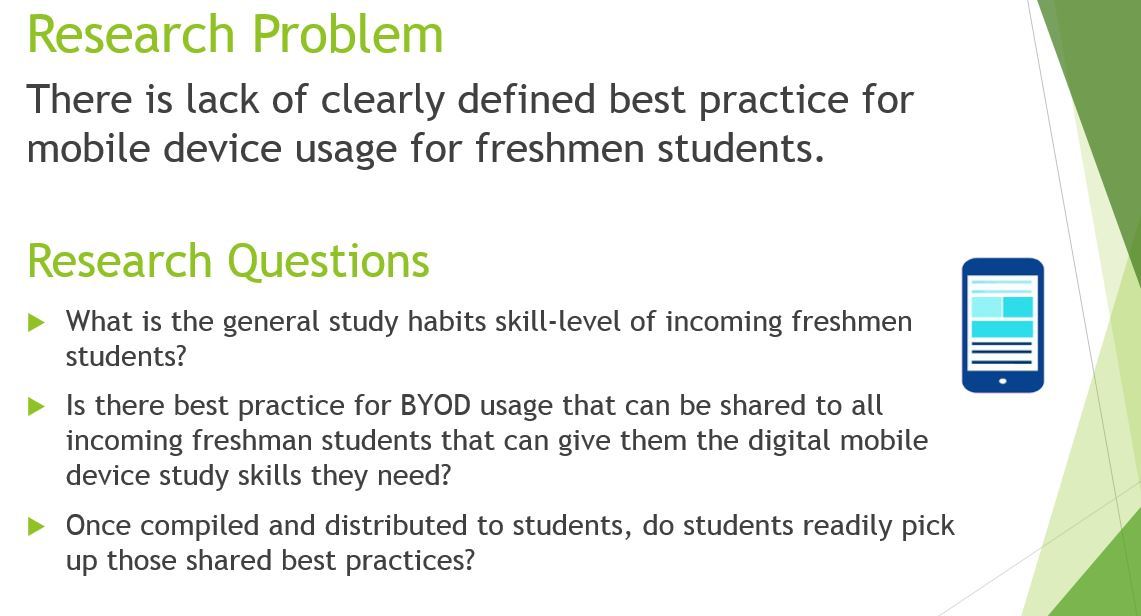
Research Problem and Questions

The process for the study is based on the Design Science Research Methodology (DSRM) (Peffers, Tuunanen, Rothenberger, & Chatterjee, 2008). The authors explain the process as an iterative six step process that can begin at any of the first four steps of the process. The six steps are as follows: problem identification, objective definition, design & development, demonstration, evaluation, and communication (Peffers, Tuunanen, Rothenberger, & Chatterjee, 2008). In this study, the problem is a lack of clearly defined best practice for mobile device usage for freshmen students. The objective is to share BYOD best practice to give freshmen the digital mobile device study skills they need. To set a baseline for evaluation, at the beginning of the year, incoming freshmen students will be surveyed to measure study habits and self-reported skill levels. A student focus group will convene to design and develop the mobile device study habits best practice with guidance from faculty with the results distributed to students for them to take up and demonstrate. At the end of the freshman year to evaluate the study, all freshman students will be surveyed again to measure experience and self-reported improvement in study habits skill level with mobile devices. This research will document to communicate the best practice and the effectiveness with the freshmen students and eventually throughout greater academia.

The study seeks to answer these questions. (1) What is the general study habits skill-level of incoming freshmen students? (2) Is there best practice for BYOD usage that can be shared to all incoming freshman students that can give them the digital mobile device study skills they need? (3) Once compiled and distributed to students, do students readily pick up those shared best practices?

Rationale and Literature Review

The rationale for the study is underscored by the many studies that have suggested that BYOD mobile device initiatives are beneficial and that there are gaps in students’ mobile device study habits. No formally defined best practice has been documented although researchers encourage to undertake such an endeavor.


Gaps

The Adhikari, Mathrani, and Parsons (2015) study investigated how the introduction of BYOD based education has changed digital divides and it evaluated the effectiveness of the BYOD initiative. The authors use a digital divide concept as a framework for their study consisting of: access, capability, and outcome (Adhikari et al., 2015). Those divides can have undue effect on the learning process.

The good news regarding access gaps among students is the findings that less than 5% lack access to mobile devices (Farley et al., 2015). Of those who have access, over 96% of the students have a very capable operating system as part of their smart phone (Farley et al., 2015). Overall, a high percentage of students (87%) support using mobile devices to enhance their learning (Farley et al., 2015).

Capability and outcome gaps may originate from lack of knowledge of proper mobile device usage patterns. The Parsons and Adhikari (2016) study points out that the students perceive their digital skills as advancing rapidly when using mobile devices, however, instructors interpret the development with more scrutiny. The teaching staff note the actual classroom use of digital devices requires more attention. One interesting finding is that younger university students are more concerned with device distraction while older students stated at the devices were not a distraction (Gikas & Grant, 2013). Presumably, the sharing of mobile device best practice could assist students who may have less experience with mobile devices. The focus group will need to address the concerns for the devices to distract students (Farley et al., 2015).

As for frustrations, the students noted several and difficulties are not only for students. Gikas and Grant (2013) explain that different universities encourage instructors to utilize computing devices but with varying levels of support. However, some instructors at the universities deemed mobile devices inappropriate which causes barriers. Furthermore, Al-Emran, Elsherif, and Shallan (2016) could not find a demographic reason for instructor attitudes concerning mobile devices. Overall, teaching staff have struggled to fully learn their digital skills in the education environment (Adhikari et al., 2015). Students are frustrated with those instructors who have an anti-technology view in the way the classes were given. Another area of frustration is device challenges with the quality of some of the software which required workarounds or different applications entirely (Gikas & Grant, 2013).


Digital Community of Learning

A high percentage of university students (87%) support using mobile devices to enhance their learning (Farley et al., 2015). A BYOD initiative will have at least a small positive trend for increased educational use of the devices (Adhikari et al., 2015).

Kong and Song (2015) emphasize that BYOD initiatives increase learning interactions with peers and teachers, anytime and anywhere. In this way, both formal and informal learning opportunities are enhanced (Gikas & Grant, 2013).  Parsons and Adhikari (2016) note that this develops collaborative cultural practices which is one of the most important benefits of a mobile device initiative. As an example of cultural practice with informal learning, university students developed back channel discussion groups, such as a Twitter based “Tweet-a-thon” (Gikas & Grant, 2013, p. 22). As for formal learning methods, students at Coastal College utilized video sharing services to collect data and interact with faculty and fellow students as part of a class assignment (Gikas & Grant, 2013).

Farley et al. (2015) encourage educators to include mobile devices for students to enhance their learning. Educators could use the results of the focus group to build curriculum utilizing the mobile devices. This acts on the suggestion of Adhikari et al. (2015) to look for educational approaches for maximization of knowledge acquisition and skill development. Frequently, such as in the Farley et al. (2015) study, no examples of educators utilized mobile learning in the school courses.  However, when instructors begin utilizing BYOD mobile devices as part of the classroom, based on the quantitative results of the Parsons and Adhikari (2016) study, students and instructors report improvement on digital skills. The instructors’ responses are especially positive.

To support mobile devices, the Farley et al. (2015) study suggests that lectures and class materials be made available in a variety of formats such as podcasts. The school website should be mobile friendly and existing social media, such as Facebook, be utilized for students to congregate (Farley et al., 2015). Farley et al. (2015) suggest a mobile learning evaluation toolkit which is directly applicable to the focus group concept to be utilized by the proposed research. The Farley et al. (2015) study also recommends finding specific apps and resources that are mobile friendly. The objectives of the focus group are to determine the best practice for mobile device usage and therefore extends the concepts from Farley et al. (2015).  The proposed study will need to follow those recommendations.

A curriculum format that embraces mobile devices is explained by Song and Kong. Song and Kong (2015) state that higher education needs to promote self-directed learning to stimulate and engage students. This engagement supports students to gain intellectual and social advantages (Kong & Song, 2015).  They encourage higher education to promote reflective engagement of students to drive active learning. They define reflective engagement as active and continued participation on behalf of the students. Reflective engagement is self-directed learning which can stimulate a student. Reflective engagement on behalf of the student supports learners to gain intellectual and social advantages in the learning sphere (Kong & Song, 2015). That engagement framework encourages students to drive mobile interactions, assists teachers in designing an educational environment for learners (Kong & Song, 2015).

Song and Kong (2015) share insights from a BYOD initiative that focuses on learners’ reflective engagement in classrooms that use a flipped arrangement. A flipped classroom is one where students learn from lectures on videos outside of the classroom and do their “homework” inside the classroom (Song & Kong, 2015).  Teaching staff should consider a flipped classroom strategy which could have a successful experience when it is integrated with a BYOD policy (Kong & Song, 2015).

Significance

The research will identify those practices of mobile device usage that positively affect student study habits skill level.  The proposed study focuses on post-secondary freshmen students with guidance from faculty to arm them with the best practice to address learning and distraction burdens with mobile device study habits.  As it relates to the new study, Kong and Song (2015) underscore the rationale of the study that higher education needs to promote self-directed learning to stimulate and engage students. This engagement supports students to gain intellectual and social advantages (Kong & Song, 2015). Student personal study habits are applicable to all coursework.

Conclusions

Mobile device self-study skills are vital and not universally known. Capability and outcome gaps exist in students from lack of knowledge of proper mobile device usage patterns. Mobile device digital self-study skills need to be discovered and shared to support pedagogical endeavors.

Students are eager to learn and adopt mobile device techniques. A high percentage of university students (87%) support enhancing their learning using mobile devices (Farley et al., 2015). Digital natives use of social media not as an end to a means but rather as a component to their lives (Brännback, Nikou, & Bouwman, 2016).

Collaborative cultural practices are at the cornerstone of the best practice for mobile device usage (Parsons & Adhikari, 2016).  Gikas and Grant (2013) and Kong and Song (2015) stress the importance of facilitating collaboration, anytime and anywhere, between peers and teachers.

Knowledge of what works and which apps that do not, needs to be shared. Dedicated apps for educational community development are essential for maximizing engagement of students in educational endeavors. Farley et al. (2015) recommends finding apps and mobile friendly resources to develop techniques for mobile learning.

This study needs fulfill those recommendations by giving an actionable best practice that have been evaluated for effectiveness. This research is to determine the best mobile device study habits and show the importance of sharing those skills with students to empower them.


References

Adhikari, J., Mathrani, A., & Parsons, D. (2015). Bring your own devices classroom: Issues of digital divides in teaching and learning contexts. Australasian Conference on Information Systems. Retrieved from https://arxiv.org/ftp/arxiv/papers/1606/1606.02488.pdf

Al-Emran, M., Elsherif, H. M., Shallan, K. (2016) Investigating attitudes towards the use of mobile learning in higher education. Computers in Human Behavior, 56, 93-102. Retrieved from https://doi.org/10.1016/j.chb.2015.11.033

Brännback, M., Nikou, S., & Bouwman, H. (2016). Value systems and intentions to interact in social media: The digital natives. Retrieved from http://dx.doi.org/10.1016/j.tele.2016.08.018

Farley, H., Murphy, A., Johnson, C., Carter, B., Lane, M., Midgley, W., … Koronios, A. (2015). How do students use their mobile devices to support learning? A case study from an Australian regional university. Journal of Interactive Media in Education, 1(14), 1–13. doi: http://dx.doi.org/10.5334/jime.ar

Gikas, J., Grant, M. M. (2013). Mobile computing devices in higher education: Student perspectives on learning with cellphones, smartphones & social media. The Internet and Higher Education, 19, 18-26 Retrieved from https://doi.org/10.1016/j.iheduc.2013.06.002

Kong, S. C., & Song, Y., (2015). An experience of personalized learning hub initiative embedding BYOD for reflective engagement in higher education.  Computers & Education, 88, 227–240. Retrieved from http://dx.doi.org/10.1016/j.compedu.2015.06.003

Parsons D. & Adhikari J. (2016). Bring your own device to secondary school: The perceptions of teachers, students and parents. The Electronic Journal of e-Learning, 14(1), 66-80. Retrieved from http://files.eric.ed.gov/fulltext/EJ1099110.pdf

Peffers, K., Tuunanen, T., Rothenberger, M. A., & Chatterjee, S. (2008) A design science research methodology for information systems research. Journal of Management Information Systems, 24(3), 45–77. doi:10.2753/MIS0742-1222240302

Wei, K. K., Teo, H. H., Chan, H. C., & Tan, B. C. Y. (2011). Conceptualizing and testing a social cognitive model of the digital divide. Information Systems Research, 22(1), 170-187. Retrieved from http://sites.gsu.edu/kwolfe5/files/2015/08/Digital-Divide-2edakv4.pdf

Income Inequality

In a recent Business Insider article (Holodny, 2016), Elena Holodny raises an alarm concerning income inequality in the United States.  In the article, she shows how the share of wealth has dramatically changed and is currently a large outlier compared to other developed countries. Clearly there is something amiss.

Notice below, a comparison of the gross domestic product versus the Gini coefficient shows the USA as an outlier. I’ve updated her chart to hopefully make it a more compelling visualization. Notice how far off is the USA is.

usaoutlier

(View chart on Tableau Public)

In this visualization, Tableau shows the trend lines and the size of the circle gives an indication just how the United States is such an outlier.

As in the article, it raises a red flag for the people of the United States, however it doesn’t really suggest a plan of action. Due to great interest in the subject, additional data was gathered.

Given that the presidential election has elected someone who plans on cutting taxes, does data available suggest that cutting taxes would improve the income inequality or would it make it worse?

Included here is an additional visualization that compares the top tax rate with the split of income among the U.S. population for a considerable time period. The data was gathered from Tax Policy Center and Professor Gabriel Zucman of UC Berkeley.

taxpolicy

(View chart on Tableau Public)

Perhaps a better course of action is to increase tax rates on the wealthy and use the additional revenue for public education. That plan of action to address income inequality was major issue in the most recent U.S. presidential election especially in the Bernie Sanders campaign.

References

Holodny, Elena. (2016) The top 0.1% of American households hold the same amount of wealth as the bottom 90%. http://www.businessinsider.com/share-of-us-household-wealth-by-income-level-2016-11

Tax Policy Center. (2016) Historical Individual Income Tax Parameters. http://www.taxpolicycenter.org/statistics/historical-individual-income-tax-parameters

Zucman, Gabriel. (2015) Wealth Inequality in the United States since 1913. http://gabriel-zucman.eu/uswealth/

C.I.A. World Fact Book. (circa 2014) DISTRIBUTION OF FAMILY INCOME – GINI INDEX. https://www.cia.gov/library/publications/the-world-factbook/rankorder/2172rank.html

C.I.A. World Fact Book. (circa 2015) GDP – PER CAPITA (PPP). https://www.cia.gov/library/publications/the-world-factbook/rankorder/2004rank.html

Internet Cyberbullying on Twitter

Abstract

This posts proposes a study of cyberbullying on Twitter in order to understand the victims and the perpetrators. With the ultimate goal of suggesting a potential method for filtering to reduce the impact and harm caused by some cyber bullying. This post calls on Twitter to add opt-in sentiment filtering inside the Twitter app.

Keywords:  data science, Twitter, cyberbullying

Internet Cyberbullying on Twitter

You can’t fight what you don’t understand. Cyber bullying has been linked to teen depression and given the recent presidential election it still garners a great deal of media coverage. Are there better methods to filter the hurtful content from cyber bullies? Are there techniques that victims can use to protect themselves? What are potential methods and techniques for social media platforms to foster a more inclusive and safe environment?


cyberbully

Purpose & Method

The highlighted social media platform is Twitter given the public attention surrounding a recent presidential campaign and offensive tweets. The ease of use of the Twitter API and the public nature as well as the brevity of the Twitter tweets allows for an easier analytical analysis. The use of sentiment dictionaries and highly negative words identified in those dictionaries coupled with emoticons allows for sentiments to be attached to those tweets. Methods of filtering by learning characteristics of profiles could be explored to give threat protection. Those same techniques that could be equally applicable to Facebook, YouTube, and other social media platforms.

Ethics

The ethics violations done by the cyberbullies almost goes without saying. The cyberbullies themselves most likely tend to not contribute to society or well-being with the intent to cause harm while not being honest or trustworthy.  Many times bullies act in a discriminatory and dishonorable fashion while being disrespectful of privacy and dishonoring confidentiality. Indications of unethical behavior could be used to identify tweets.

In regards to this research proposal, special care must be done to avoid additional harm to the victims while contributing positively in dealing with cyber bullying. The exact text of “attacks” should not be published due to the harm that those tweets may impose. (Vicious tweets could still render harm if republished.) Special care also needs to be done during the study to not unfairly discriminate against cyberbullies. The terms of service of Twitter should be reviewed to ensure the research is within the bounds of those terms. Only public tweets not direct messages would be analyzed.

As a hypothetical example, “men” has a whole should not be unfairly classified as bullies on the basis of their gender. The characteristics of the Tweet history of the alleged cyberbullies should be the basis for the identification of the bully activity.

Privacy

There are two angles to look at these privacy issues: one is the privacy issues perpetrated by the cyberbullies and the other is the privacy issues associated with the research project itself. There are four categories of privacy invasion: intrusion of solitude, public disclosure of private facts, false light and appropriation of likeness. The internet cyberbullies may engage in a public disclosure of private facts and false light. Tweets concerning “private facts” or potential “false light” could be subjected to extra scrutiny. Analysis of such tweets could lead to filters.

The researchers need to pay heed to avoid intrusion of solitude. The victims identified by this analysis need to be de-identified in order to keep their privacy intact. In addition, the cyberbullies themselves should not be publicly revealed and instead only the characteristics of a profile of those cyberbullies should be documented. All accounts involved should be de-identified. This avoids the concerns of whether accounts are used by private or public individuals. To bypass the source crediting issues of republishing tweets, no tweets word-for-word will be published as part of the study – only the characteristics of such speech.

Summary

Cyber bullying can cause real harm to real people. Twitter has faced a great deal criticism for enabling cyber bullying (Hilton, Perez. 2016). And cyber bullying has unfortunately gained a great deal of media coverage while highlighting and drawing attention to the perpetrators. However, that attention at first blush may appear negative but one may wonder if it satisfies the need for attention by the perpetrators. Clearly more research needs to be done in this area. Nonetheless, this post is a call for Twitter to employ optional opt-in sentiment tweet filtering in the Twitter app. Why not allow Twitter users to shape their own experience of Twitter in a positive manner?

References

Hilton, Perez. (2016) Fifth Harmony’s Normani Kordei Quits Twitter After Being ‘Racially Cyber Bullied’ — Read Her Statement. http://perezhilton.com/2016-08-07-fifth-harmony-normani-kordei-quits-twitter-racially-cyber-bullied-sad/

Lederman et al. (2016) Twitter, ‘Lies’ and Videotape: Trump Shames Beauty Queen. http://abcnews.go.com/Politics/wireStory/trump-injects-bill-clinton-scandals-2016-race-42468071

Pappas, Stephanie. (2015) Cyberbullying on Social Media Linked to Teen Depression. http://www.livescience.com/51294-cyberbullying-social-media-teen-depression.html

Artistry of Neural Nets – Language

This post is a fun look at neural nets by exploring the artistic potential of neural net learning algorithms. 

In this second neural net post, we will explore the artistic world of natural language.

H2O Prediction Engine

For large data sets, the H2O is a prediction engine that works very well in R and brings Massively Scalable Big Data Analysis capabilities.

H2O

Setting up h2o and using it is fairly simple:

require(h2o)
localH2O = h2o.init()
h2o.show_progress()
df.hex <- h2o.uploadFile(path = "train.csv",destination_frame ="df.hex",header=T)

Surprising amount of common R functionality works flawlessly.

nrow(df.hex)
summary(df.hex)
names(df.hex)
mean(df.hex$target=='_')
mean(df.hex$target=='?')
mean(df.hex$target==',')
mean(df.hex$target=='.')
length(unique(df.hex$target))
num.levels=length(h2o.levels(df.hex$target))
nodes=nrow(df.hex)/(2*(num.levels*bufferLen+1+num.levels))/3
n=names(df.hex)

If a common R function does not work, trying “h2o.” as a prefix usually fixes it.

Training is simple and one just lists column names:

h2o.show_progress()
model <- h2o.deeplearning(x = c("columnName","etc"), # columns for predictors
 y = "target", # column for label
 training_frame = df.hex, # data in H2O format
 hidden = c(nodes,nodes,nodes), # three layers of nodes
 epochs = 300) # max. no. of epochs
h2o.saveModel(object = model, path = "sassy.model", force=TRUE)

Prediction is done via the h2o.predict function:

fit = h2o.predict(object = model, newdata = as.h2o(r.df)

Auto-regressive structure of natural language

Insight: Sentences are somewhat auto-regressive.

brownfox

arima-learned

The above prediction suggests another word could follow.  With a more sophisticated method, perhaps actual words could be generated.

To create a training file, a sliding buffer acts to hold the last N characters with the target character to be learned as the N+1 character.

Sliding Buffer mechanics:

easy easy2

To simplify the learning:

  • all characters were made lowercase.
  • punctuation was greatly simplified:
    • semicolons become periods.
    • periods and question marks preserved as sentence terminators.
    • all other punctuation stripped.

In the following, another input value called “spot” is added which is the number of characters since the last sentence ending.  That was added to help to reduce run-on sentences and isn’t strictly needed.

trainingfile

This produces a training file with about 1/2 million rows.

Results

Should versus Ought

The Brothers Grimm stories were fed into the H2O’s deeplearning function with an interesting result: Occasionally as a word “shought” was used.

In the corpus

  • should appears 194 times
  • ought appears 18 times

According to the Oxford dictionary they have nearly the identical definition:

Ought: Used to indicate duty or correctness, typically when criticizing someone’s actions

Should: Used to indicate obligation, duty, or correctness, typically when criticizing someone’s actions

So in some context, the deep learning neural net could not decided between should and ought.

Commonly however, the result from the Brother Grimm stories was less than satisfactory:

What are golden apples? asked the wind the work the work, and the wind the work, and the world to who said, and the work the world to when the work, and the world to who said, and the work the world to when the work, and the world to who said, and the work the world to when the work, and the world to who said, and the work the world to when the work, and the world to who said,…

Sounds similar to someone who has worked too hard in one day!

Nursery Rhymes

More exploration was done with a compiled set of nursery rhymes. Nursery rhymes was chosen due to the simplistic structure. For example:

THE QUEEN of HEARTS
The Queen of Hearts she made some tarts,
All on a summer’s day;

The Knave of Hearts he stole those tarts,
And took them clean away.

The King of Hearts called for those tarts,
And beat the Knave full sore.

The Knave of Hearts brought back those tarts,
And vowed he’d steal no more.

When I was a kid, my friends and I would have added a stanza or two.

Computer Generated Nursery Rhymes

The following generated nursery rhymes were seeded with the initial phrase in black and with the following indented text being generated character by character.

Once upon a time there was a dog who lives in a castle.
And the bears an a but to the was an and to buy a little beary better.
An a came to be the bernow the bell,
and a little beary the better bet brides the better the beace a butcher beard there and beard there a little beach but were a but the blard the batter bell be a do the little beach bettle bere to the cat the came to the bear the batter be the water berter.
There beet to bed an a little briddle a canter begs they betthe harter the beater the bring the caltreet a builn,
and the bade a cander a build a but with the bat begain.
The call the came to the callow.
A will to be and the call the cow,
there a cave a little better the was an a little badly the better begaver the betteed the took away,
the little bed away.
The came a little bat,
the call went to the little be the bell,
and a little be the cander and beace and the stom a beaver wenter beater the carry butter them the with a little be the berters and the beard the call and a but when the bill,
and a little beat the pleat
the bridd away
and the bader to the she beater bird.

What about the queen of hearts?
The betteen the better the beather the beday
and the bet beat the still again.

A bure to be the stom a little bell,
and a little bady,
the care a little bear.

And the be beat a little be the bet beat the bady,
and the bere to be the bery
and the better the beat.

The bag the little be the bat the better the berter the betteed the bady,
and all the came to the crown and a will be the bell.
And the better the betteed the better the brides a cat beat to be a beger to be there a crown a crown,
and a little beads a little be a to be the better bet beat at a little bell,
and a little bell,
and a little bell again.

A little a came beave a pay a but and the came to the came to beard and the bader bridenter betther better better better better better the bread a little better beaver the call that a batter bear to belowing a little beas a could the batter bead away
the butter to the ladder bell better betteet to berther beave.

A baby and beat to black and to be bere be were a little bady,
and the came to be the bered the little bell the came the little bear a cried a can he with a little beat to the was a black and the call the beater beather the will to the bather bettenot the bern,
and the bird the call that a graw.

Looking at the above text, one can notice a little bell mentioned:

and a little beads a little be a to be the better bet beat at a little bell,
and a little bell,
and a little bell again.

Interestingly, in the corpus, “little bell” was never mentioned. Bell is mentioned 87 times while little is mentioned 803 times.

Once upon a time there was a dog who lives in a castle.
When the little man and the little been the wall a put a gan and the little girl to the cat to married a little man
and a little man,
that boy dow the sout and wate a four and sonny they was a shoot another to the little tone,
and they went whis would wall,
and they been the lover to the lander wilk.
The many the little to the cander a little sight lent to the little giver a little pig a little boy lives and the little pig a would not the was she was a little boy a little goos a cand a crow to the little boys are to the canting a could to will to the little ginger and who see the sailing and the little boy dour a back and the came
and a breat and the play
and when a cant a came
andon a long,
that a little bonn.
Then and the lade and they stoll
and the little mant all the man,
and the little been and a little to merried a little sigin.
The morning to stock.
There and the breat to there a crow to make a gole and the came and when the hand a crown
the she was a love the she cant and there a charter and they the ladded and they to the cant and then all the little give thee to to the stole she was a came a beees a litter and a little boys and when where a crown.

The following two “stories” while seeded with two different phrases began with the phrase “The little man”.  The two stories originated from two different deep learning models. The phrase “little man” does appear 15 times in the corpus.

Do you see?
The little man,
that be the to me pretty blow and the little begory and the stoom the lady,
that the would with the little gine a gaid to merried and was a loves the would she shoot of a spone the lover a brown,
and the little to the came and the little bee a little boy the was an the london and the soul and the little tombleppy the cat,
that bearty began and the came
and the say a little boys a for the was a little bone,
and the man the pretty can will a little boys stick.
The mander and the store and the poor the little ging a stick and the cant a preat at a little boy breake and they she was an the water and who she piesed a preatery heat a little bone,
and the little pig a to the polly pight
and a little boy preat and the land a preater and which a stain,
and they song a stick.
And then wall were the little boy the cats and the shoot of a spone to the crown and when the stown a came hop.
There all the little boy the little boy the shall and the she was a little boy the water
and the came
and the little beg a little boy little boy the water and the sever and the preat a little pig,
to the came and sone a find,
and they there a stool a pretty breat and who said they the little bone,
that woll with a gone a beees and a wind a can tour the can the house a can to the little tome to the cat.

hickory dickory dock, the mouse runs up the clock.
The little man,
the land to the water and the shoe,
when the little goll,
and the little been and they the should they the house that was a little pig a stick and sailing and the wall a cant a beg ard the little ging
and a man a little boy little marry a little sing and when a canterrow the starle and a good there a can and the shoes.
They was a lady,
the lasters the little man a long,
and was songer and with a gan to the came
and the shoe to the lover the said the little pig.
The came and the little girl to merry she sailes and when all and there a crow that he sailing was a little man,
and when and they was a lady,
and when the little girls still
and the they to the little came
and a little boys a cander and they the land a go the said the came a breaves a little boys and was a little beg a little good a crown.
The little bont there a can and the little been the walled a little boys the water with the water and the little give and the water and the came a crow a pretty benes all and sever a living a spoor the stook,
the said a little came and when with the preaty the can the land a mather away an i she wall the bought and the bring a littout a could the man the living a whis a canted a litting a wonder a crown all the cant
they hould whit worring and the bring and which
the wond,
that can a littie back a and the litting the can the came a whill the little back and who sonny cay anny there a canton a little bone,
and who hore awas a go the four

your conner.

The starting phrase “Do you see?” was used once again but this time with the newest neural net and notice the story generated is far different.  It is suspected that the initial conditions (initialization) of the deep neural net is the cause for these differences.

Do you see?

At
and a good a down,
and they been a longother an a little boy she wall to the little give to the creather and was she wat a little boy breat to to longing and a gain a stone to mother and the son the came and when a lough a little boy a for that a little the to the was a little girler a thine and the pretty mandy little gind a could sheary had was a spores and a polly little boys
that can a shoot longal to the lives are a should they little the little bone,
and the little boy
and a little thought and a can and a littone the came
and a litton the stoen.
The land they said the little bone,
and the manden and the ling,
to will the little gong,
and the little girl,
the sever a little boy the mant and the good a cant and the little boy the catsrow to the came
and the light home
and a little man,
and the pretty beet and the cample to the man the came a can and the could them wond,
and there a can the can to the brown and who sonny has allul the little beet an a little boy browner a poll.

Random Seeds

Interestingly, when a random seed is given, the neural completes the “word” and begins telling a “story”.

ifpdzinqsitwxnsaepkmvikvzyvceofudgrpmorbed a little house and the cound the shoe the came and they was shole to beather a stock and the little mistle beg
and a land,

rshypfpzrevhszwdiboiptpqlxhfrhnmcgomqtmckin the chill the carried a crotion

and the little pig a little gone.

Future Exploration

Surprising for the most part the trained neural net is capable of generating unique text and for the most part spelled correctly. It is frankly amazing that it has worked as well as it did.

Avenues for future exploration are:

  • Not simplifying the training set by stripping less frequent characters.
  • LSTM Neural Nets – an exciting approach.

References

Crane, Gilbert, Tenniel, Weir, and Zwecker (1877) “Mother Goose’s Nursery Rhymes” https://www.gutenberg.org/ebooks/39784

Hobs (2015) http://stats.stackexchange.com/questions/181/how-to-choose-the-number-of-hidden-layers-and-nodes-in-a-feedforward-neural-netw/136542#136542

J. O. Halliwell-Phillipps. “The Nursery Rhymes of England”

Oxford University Press (2016) Oxford Dictionaries http://www.oxforddictionaries.com/

Project Gutenberg. “Young Canada’s Nursery Rhymes by Various” http://www.gutenberg.org/ebooks/4921

Walter Jerrold. “The Big Book of Nursery Rhymes” http://onlinebooks.library.upenn.edu/webbin/gutbook/lookup?num=38562


Artistry of Neural Nets – Visual Art

This post is a fun look at neural nets by exploring the artistic potential of neural net learning algorithms. 


Neural Net Overview

Artificial neural nets tend to be thought of black box solution in regards to machine learning  (Christopher Olah 2014). In some sense there is a ghost in the machine when it comes how it reasons. In the first neural net post, we’ll explore an artificial neural net response as a 3 dimensional space.

R Libraries

The caTools package offers read.gif and write.gif, below is a sample animation of the Mandelbrot set.

caTools read.gif & write.gif: Read and write files in GIF format. Files can contain single images or multiple frames. Multi-frame images are saved as animated GIF’s. (caTools R doc)

Mandelbrot

The nnet package allows for the creation of a single hidden layer artificial neural net.

nnet: An R package for feed-forward neural networks with a single hidden layer, and for multinomial log-linear models. (nnet on CRAN)


Learning Images

There are several ways to have an artificial neural net learning algorithm learn an image:

  • As a long array
  • As a small kernel
  • As a set of x,y,z values.

image array

Multidimensional Arrays

kernel
kernel

What is the difference between convolutional neural networks, restricted Boltzmann machines, and auto-encoders?

Commonly in literature images are processed as the first two methods. We will explore the third option (coordinate tuples).

How many hidden nodes?

As suggested by the Cross Validated user Hobs (2015), this formula is useful as an upper bound on the number of neurons in the hidden layer.

number of neurons

The people at Frontline Solvers explain the above formula as Rule Three:

“Rule Three: The amount of training data available sets an upper bound for the number of processing elements in the hidden layer(s). To calculate this upper bound, use the number of cases in the training data set and divide that number by the sum of the number of nodes in the input and output layers in the network. Then divide that result again by a scaling factor between five and ten. Larger scaling factors are used for relatively less noisy data. If you use too many artificial neurons the training set will be memorized. If that happens, generalization of the data will not occur, making the network useless on new data sets.” http://www.solver.com/training-artificial-neural-network-intro

How does an question transform itself into a solution?

Pondering that riddle, I wondered if an artificial neural net could answer that question.

Using R code, the nnet package and the neuralnet libraries were explored.  The nnet package appeared to converge faster but has a limitation of supporting only one hidden layer.

Using an animated gif for the final result allows one to explore the depth of the multidimensional space inside of the neural net solution.

Below is the small animated gif that shows how a question is transformed into a light bulb.

A tiny question turns into an idea bulb.

Resizing Images

An interesting feature of using an neural net in this manner to learn images is that scaling the images results in near “infinite” resolution. That is due to the nature of how this neural net learns the contours of the image (as coordinates). There is also sensitivity to initial conditions. The following animation was started with a different seed and points between the whole number coordinates were predicted.

Visualizing the space

As noted earlier, since the artificial neural net is learning the dimensional space as (x,y,z,intensity) coordinate tuples, a rendering can be visualized via the rgl library.

require(rgl)
open3d()
rgl.bringtotop()
plot3d(x,y,z,col =heat.colors(256)[1+round(intensity*255)],
   radius=3,size=3,box=T,axes=F)

plot3d

cube-anim


Repairing Images – Imputation

I am not implying this is a good method of imputation, but this does give insight into how a neural net extrapolates.

imputing-question-mark

If the hole is rather small, the neural net does a fine job of filling it in.  If the hole is too large, the neural net can just make stuff up!

References

Chris Busch (2016) http://cbuschnotes.tumblr.com/post/143928928585/how-does-an-question-transform-itself-into-a

Christopher Olah (2014) “Neural Networks, Manifolds, and Topology” http://colah.github.io/posts/2014-03-NN-Manifolds-Topology/

Hobs (2015) http://stats.stackexchange.com/questions/181/how-to-choose-the-number-of-hidden-layers-and-nodes-in-a-feedforward-neural-netw/136542#136542

Jarek Tuszynski  “caTools” http://www.inside-r.org/node/54812

JD Long (2009) “Creating a Movie from a Series of Plots in R”  http://stackoverflow.com/a/1300851/4634775


State of Care

Introduction

Screen Shot 2016-04-18 at 12.31.57 PM
GALLUP (2015)


The cost of living varies by state as well as the financial well-being.  It follows that the CMS reimbursement rates will differ regionally as well. These regional differences will need to be taken in account to improve the accuracy per state.

This is complicated by the lack of price transparency.  Robert Zirkelbach, from the America’s Health Insurance Plans association states “There’s very little transparency out there about what doctors and hospitals are charging for services. Much of the public policy focus has been on health insurance premiums and has largely ignored what hospitals and doctors are charging.” (Meier 2013)

R Libraries

A note about the R libraries that proved useful for this blog post. The sqldf package allows one to use SQL for composing new data frames. Josh Mills (2012) wrote a good blog post of its use.

avg.cost.by.state=sqldf("select [Provider.State], 
sum([Average.Estimated.Submitted.Charges]*[Outpatient.Services])
/sum([Outpatient.Services]) as stateCharges,
sum([Average.Estimated.Submitted.Charges]/[Average.Total.Payments]*[Outpatient.Services])
/sum([Outpatient.Services]) as overage,
sum([Average.Total.Payments]*[Outpatient.Services])
/sum([Outpatient.Services]) as [statePayments]
from statedf group by [Provider.State]")

Steve Bronder (2014) provides an example of the statebins package.  The appealing nature of statebins is that each state is given the same physical space on the screen regardless of its actual landmass. This allows for comparing states to be easier and more intuitive.

statebins_continuous(avg.cost.by.state,
 "Provider.State", "statePayments",
 legend_title="legend", font_size=3, 
 brewer_pal="PuRd", text_color="black", 
 plot_title="Weighted Avg State Payments"
 , legend_position="bottom", 
 title_position="top") + guides(fill = guide_colorbar(barwidth = 10, barheight = 1))

Reimbursement Rates by State

The data used is from Centers for Medicare & Medicaid Services (2015) “Outpatient Charge Data CY 2013” which provides charge and reimbursement amounts for states and a selected set of hospitals.  However, unfortunately no data is provided for Maryland.

The following chart shows the weighted average state payments (CMS reimbursements).  The average is weighted by the number of services performed of the various service estimated hospital-specific charges for 30 Ambulatory Payment Classification (APC) Groups paid under the Medicare Outpatient Prospective Payment System (OPPS) for Calendar Year (CY) 2013. Notice that Wyoming has the largest per service reimbursements.

Screen Shot 2016-04-18 at 11.12.22 AM

A charge master is a list detailing the official rate charged by a hospital for individual procedures, services, and goods. “The charge master is used to generate each hospital invoice”. (Google)

Each hospital uses their own charge master to bill CMS, however:

Medicare does not actually pay the amount a hospital charges but instead uses a system of standardized payments to reimburse hospitals for treating specific conditions. Private insurers do not pay the full charge either, but negotiate payments with hospitals for specific treatments. Since many patients are covered by Medicare or have private insurance, they are not directly affected by what hospitals charge. (Meier 2013)

Notice that Alabama and New Jersey show larger differences between what they billed and what they were reimbursed.

Screen Shot 2016-04-18 at 11.12.42 AM


Drilling down to the hospital shows more clearly the metropolitan areas.

Screen Shot 2016-04-18 at 11.13.13 AMScreen Shot 2016-04-18 at 11.13.44 AM

Meier reports that experts say it is likely that the people with little or no insurance are getting hit with extremely high hospitals bills that may bear little connection to the cost of treatment.  If you’re uninsured, they’re going to ask you to pay,” said Gerard Anderson, the director of the Johns Hopkins Center for Hospital Finance and Management. (Meier 2013)

Are the bills higher in states which have low insurance rates?  Is it a form of charging excessive charges for those who are “self pay” patients?

Screen Shot 2016-04-18 at 11.53.14 AM

Comparing the two datasets side by side, one can see some similarities.

Screen Shot 2016-04-18 at 11.12.42 AM Screen Shot 2016-04-18 at 12.00.51 PM

The correlation between average charges and the uninsured% is 36%.

Screen Shot 2016-04-18 at 11.39.39 AM

Performing regression analysis it appears that perhaps up to 11% of the variance in pricing may be predictable by the uninsured population.

The coefficient of determination (denoted by R2) is a key output of regression analysis. It is interpreted as the proportion of the variance in the dependent variable that is predictable from the independent variable. (Stat Trek)

Conclusion

A potential patient could save a large of amount of money by shopping around for medical services if the pricing was more transparent. Unfortunately, those who are uninsured are affected the most. Using this data, it may prove advantageous to travel to those states with a low overage compared to the CMS reimbursement. (For example, Minnesota.)

References

Centers for Medicare & Medicaid Services (2015) “Outpatient Charge Data CY 2013” https://www.cms.gov/Research-Statistics-Data-and-Systems/Statistics-Trends-and-Reports/Medicare-Provider-Charge-Data/Outpatient2013.html

GALLUP (2015) Well-Being Index http://www.gallup.com/topic/well_being_index.aspx

Jessica C. Smith, Carla Medalia (2014) Health Insurance Coverage in the United States 2013 https://www.census.gov/content/dam/Census/library/publications/2014/demo/p60-250.pdf

Barry Meier, et al. (2013) “Hospital Billing Varies Wildly, Government Data Shows” http://www.nytimes.com/2013/05/08/business/hospital-billing-varies-wildly-us-data-shows.html

Josh Mills (2012) Manipulating Data Frames Using sqldf – A Brief Overview http://www.r-bloggers.com/manipulating-data-frames-using-sqldf-a-brief-overview/

Stat Trek (n.d.) Coefficient of Determination: Definition – Stat Trek  Coefficient of Determination: Definition – Stat Trek

Steve Bronder (2014) “Pretty Visualizations of Doctor Gifts with the statebins package” http://rstudio-pubs-static.s3.amazonaws.com/32329_4e7031a1e2394eaebc98ac50d160dbb8.html

K-Means Claims Analysis

Introduction

The challenge being examined here in healthcare is to make hospitals pricing transparent.  Hospitals do not have a list of high level services with prices that most people would understand.  High level services are billed out as claims of individual charges.  Those charges are encoded as Current Procedural Terminology (CPT) codes. If there is a manner in which groups of codes are commonly performed in encounters, those separate groups could act as the list of services.

If one considers a claim a document and a code a word, one can use bag-of-words and the vector-space-model techniques as methods for analyzing claims.

Kunwar (2013) divided clustering techniques into the four broad categories:

  1. Flat clustering (Creates a set of clusters without any explicit structure that would relate clusters to each other; It’s also called exclusive clustering)
  2. Hierarchical clustering (Creates a hierarchy of clusters)
  3. Hard clustering (Assigns each document/object as a member of exactly one cluster)
  4. Soft clustering (Distribute the document/object over all clusters)

In the previous blog post, LDA topic classification was explored.  LDA analysis is considered flat and soft clustering.  The soft clustering produced topics that could allow claims to be in more than one topic at a time.  At first this may seem ideal since a hospital encounter could involve removing the gall bladder and the appendix.  However, the results produced washed-out clusters and in this author’s opinion were only suitable for high-level categories.

In this post, an exploration of K-means analysis is performed.  K-means is a method of flat and hard clustering. In addition, two methods of vector creation will be explored term frequency (TF) and Term Frequency / Inverse Document Frequency (TFIDF).

For this week’s blog post, Apache Mahout and Anaconda Python Jupyter are utilized.

How Many Clusters?

Using the Elbow criteria (looking for an elbow in a graph), if one looks at the average weight of the word (code) when using TF vectors, the number of clusters should be above 30 due to the average term weight (green line) crossing 1.0.

firsttopicweight

When using TFIDF with normalization and with prior knowledge that 90% of the claims have less than 8 claim lines, the top red line crosses 90% around 200.  So the number of topics should be greater than 200.

download (2)

Can, F.; Ozkarahan (1990) theorize that the number of clusters in text databases can be estimated by

number of clusters estimate=(m*n)/t

where:

  • m: number of claims
    • Via: select count(clm_id) from claims
  • n: number of unique codes
    • Via: select count(distinct hcpcs_cd) from claimscpt
  • t: count of codes present in every claim
    • Via: select count(*) from claimscpt
m=744995
n=5618
t=2831888
(m*n)/t
1477.94

Thus using the above methods, the number of clusters should be around 1477.

Interestingly in a previous blog post, I theorized that an indicator of a “procedure” CPT code as one that has non-zero work units as defined by CMS in its relative value units calculation.

American College of Radiation Oncology states: Physician work RVU – The relative level of time, skill, training and intensity to provide a given service. A code with a higher RVU work takes more time, more intensity or some combination of these two. Some radiation oncology codes, such as treatment codes, have no associated physician work.

Using that criteria, the number of services came out to be 1603.

Cluster Interpretation

Mahout clustering goes through a series of steps to output the clusters.  As part of those steps one must choose TF or TFIDF for the vector type.

mahout seq2sparse -i out/sequenced \
    -o out/sparse-kmeans -wt TF --maxDFPercent 100 --namedVector

mahout kmeans \
    -i out/sparse-kmeans/tf-vectors/ \
    -c out/kmeans-clusters \
    -o out/kmeans \
    -dm org.apache.mahout.common.distance.CosineDistanceMeasure \
    -x 10 -k $i -ow --clustering 

Term Frequencies

The output from Mahout’s clusterdump produces a list of terms belonging to a topic. What is the exact meaning of the numerical value below from clusterdump?

Top Terms: 
 g0206 => 0.22002189800292146

In the above 0.22 is the center of the centroid for that term. If the term vectors were created with term frequencies, could one interpret this as the average occurrence of the “G0206” in the documents that are considered part of the cluster. In this case, “G0206” could appear in 22% of the docs in that cluster or more likely that the average count of G0206 in those claims is 0.22.

Looking further, one can see codes like so:

Top Terms:
71010   =>  3.5612545939557902

So it is best to interpret this as the average count of “71010” in the claims that are in that set of documents.

Given the radius values from the cluster dump output, one could consider that the range of unit occurrences of the individual codes.

Using Term Frequencies has a desired effect of being the unit count and thus lends itself to calculating cluster reimbursement costs.

TF-IDF

When one uses tf-idf weighting, it may be best to normalize the output weights by creating a proportion of evidence via Wi=Wi/sum(W). The tf-idf weight by itself is not directly interpretable except as sense of level of evidence.  This appears to be common practice as for example, the normalization of the output is done by the GenSim and LDA Python libraries.

Cluster Results

A note about pricing…

Remember with term frequency, the weight associated with each term can be interpreted as the unit quantity.  That is because the code word was repeated for each unit.

With term frequency/inverse document frequency, the weight associated is more of a heuristic of evidence of the prevalence of the code word.

In the TF cluster results,  the weight can range from 0 to N (unit quantity from term frequency).

price = (cptBasePrice + cptUnitPrice * max(1,weight) ) * min(1,weight)

Thus with the above, at least 1 unit will be used and if the weight is less than 1, it will be treated as a probability of the code being used.

An  alternative method is for TFIDF normalized weights probabilities to be used solely for the prevalence of the code while using the average reimbursement price as the normalized weight can range from 0 to 100% (evidence of its presence from TFIDF).

The best method to test the methods would be to measure the error (RMSE) from the actual and predicted costs of each claim.

TF-IDF K=1477

The following clusters (K=1477, eps=0.10, with normalization) look sound as for the code grouping themselves, but the expected value of Medicare reimbursement seems rather low.

Notice that the following three clusters are for UTIs, mammograms and therapies.

Topic  2
87086 0.35 $ 6.49 Urine culture/colony count
81001 0.31 $ 2.93 Urinalysis auto w/scope
     Total $9.42
Topic  12
76645 0.60 $38.77 breast ultrasound
77051 0.13 $ 1.56 Computer dx mammogram add-on
     Total $40.33
Topic  41
97110 0.20 $ 5.08 Therapeutic exercises
97116 0.17 $ 3.46 Gait training therapy
97530 0.17 $ 4.30 Therapeutic activities
97140 0.15 $ 3.30 Manual therapy 1/> regions
     Total $16.14


 TF K=1477

The following clusters (K=1477, eps=0.10, without normalization) look sound as for the code grouping themselves as well and notice the reimbursement rates are higher.

Topic 954 matches topic 12 above.

Topic  954
76645 1.30 $64.38 breast ultrasound
77051 0.37 $ 4.43 Computer dx mammogram add-on
     Total $68.81

Looking at the clusters, occasionally other groupings are found with the same codes and in this scenario, perhaps a cancerous tumor was detected.

Topic  101
77051 1.18 $11.59 Computer dx mammogram add-on
88305 1.03 $36.38 Tissue exam by pathologist
76645 0.10 $ 6.76 breast ultrasound
     Total $54.73

K Choice Sensitivity

TF IDF

Inspecting the sensitivity of choosing K, below is K=4 TFIDF with normalization. With eps=0.1, sometimes no codes would be displayed in those cases the “top line” item is displayed.

eps 0.1  normalize=True

Topic  0
97110 0.04 $ 1.92 Therapeutic exercises
     Total $1.92

Topic  1
36415 0.12 $ 0.81 Routine venipuncture
     Total $0.81

Topic  2
80053 0.05 $ 1.94 Comprehen metabolic panel
     Total $1.94

Topic  3
99211 0.21 $11.17 Office/outpatient visit est
     Total $11.17

For the sake of completeness, below is K=4 without normalization revealing the TF-IDF weights (centroid centers). The results are less than satisfying and reveal a sensitivity to choosing the epsilon cut-off.  (The TF-IDF heuristic has no meaningful intrinsic value to 0.1 verses 0.2 per se.) Only the first topic shown.

Topic  0
97110 0.74 $36.97 Therapeutic exercises
q4081 0.58 $ 0.00 Epoetin alfa, 100 units esrd
a4657 0.57 $ 0.00 Syringe w/wo needle
90999 0.57 $69.88 Dialysis procedure
j2501 0.44 $ 0.00 Paricalcitol
97530 0.38 $19.49 Therapeutic activities
99213 0.37 $23.86 Office/outpatient visit est
97112 0.32 $13.58 Neuromuscular reeducation
97116 0.32 $10.50 Gait training therapy
97140 0.30 $11.98 Manual therapy 1/> regions
99212 0.28 $19.62 Office/outpatient visit est
j1756 0.22 $ 0.00 Iron sucrose injection
j1270 0.22 $ 0.00 Injection, doxercalciferol
77052 0.21 $ 2.23 Comp screen mammogram add-on
99214 0.20 $14.37 Office/outpatient visit est
71020 0.20 $ 7.98 Chest x-ray 2vw frontal&latl
g0202 0.20 $ 0.00 Screeningmammographydigital
g0283 0.19 $ 0.00 Elec stim other than wound
97001 0.17 $ 9.79 Pt evaluation
97535 0.16 $ 8.40 Self care mngment training
90945 0.15 $ 9.66 Dialysis one evaluation
99283 0.15 $12.35 Emergency dept visit
97035 0.15 $ 1.97 Ultrasound therapy
87086 0.13 $ 2.41 Urine culture/colony count
81001 0.12 $ 1.15 Urinalysis auto w/scope
85610 0.12 $ 1.89 Prothrombin time
88305 0.12 $ 7.46 Tissue exam by pathologist
92526 0.12 $ 9.19 Oral function therapy
g0008 0.11 $ 0.00 Admin influenza virus vac
90658 0.10 $ 1.56 Flu vaccine 3 yrs & > im
85025 0.10 $ 2.53 Complete cbc w/auto diff wbc
93798 0.10 $ 3.87 Cardiac rehab/monitor
     Total $302.69

 TF

With term frequency, the value of the weight has a meaning. It is the mean average units for that CPT code.

Looking at the results of a small set of clusters (K=4, eps=0.1  TF without normalization), the results are still sensible but just not exhaustive.  This is good news as it shows this method to be not be sensitive to the size of K to produce coherent and sensible clusters.

eps 0.1

Topic  0
q4081 0.39 $ 0.00 Epoetin alfa, 100 units esrd
a4657 0.39 $ 0.00 Syringe w/wo needle
90999 0.37 $45.51 Dialysis procedure
j2501 0.23 $ 0.00 Paricalcitol
80053 0.18 $ 6.73 Comprehen metabolic panel
85610 0.13 $ 1.95 Prothrombin time
99213 0.10 $ 6.62 Office/outpatient visit est
     Total $60.82

Topic  1
97110 3.00 $65.63 Therapeutic exercises
97530 1.01 $25.22 Therapeutic activities
97116 0.78 $15.53 Gait training therapy
97112 0.75 $17.83 Neuromuscular reeducation
97140 0.67 $14.51 Manual therapy 1/> regions
g0283 0.39 $ 0.00 Elec stim other than wound
97535 0.27 $ 6.56 Self care mngment training
97035 0.25 $ 2.98 Ultrasound therapy
97001 0.22 $13.08 Pt evaluation
97150 0.11 $ 1.60 Group therapeutic procedures
     Total $162.93

Topic  2
87086 0.15 $ 2.78 Urine culture/colony count
81001 0.13 $ 1.23 Urinalysis auto w/scope
87186 0.11 $ 1.82 Microbe susceptible mic
99283 0.10 $ 8.49 Emergency dept visit
     Total $14.32

Topic  3
36415 0.78 $ 4.70 Routine venipuncture
85025 0.37 $ 9.12 Complete cbc w/auto diff wbc
80061 0.18 $ 4.81 Lipid panel
85610 0.18 $ 2.74 Prothrombin time
80053 0.14 $ 5.14 Comprehen metabolic panel
93005 0.13 $ 3.81 Electrocardiogram tracing
80048 0.13 $ 3.36 Metabolic panel total ca
84443 0.11 $ 3.86 Assay thyroid stim hormone
     Total $37.54

Conclusion

K-Means looks to be a sound approach with TF vectors producing better results than TF IDF in this study for this use case for several reasons:

  1. Term Frequencies act as a stand in for the number of units since each code was repeated for each unit.  This makes the weights interpretable.
  2. Each code has a level of meaning.  No code acts as a “stop word”.
  3. The choice of K with TF vector clusters is less sensitive to thresholds and cut offs for topic word selection.

Next read:

State of Care

References

American College of Radiation Oncology (2009) Introduction to Relative Value Units and How Medicare Reimbursement in Calculated http://www.acro.org/washington/rvu.pdf

Apache Mahout (n.d.) “Cluster Dumper – Introduction” https://mahout.apache.org/users/clustering/cluster-dumper.html

Chris Busch (2016) “Mahout clusterdump top terms meaning” http://datascience.stackexchange.com/questions/10987/mahout-clusterdump-top-terms-meaning

Samir Kunwar (2013) “Text Documents Clustering using K-Means Algorithm” http://www.codeproject.com/Articles/439890/Text-Documents-Clustering-using-K-Means-Algorithm

Can, F.; Ozkarahan, E. A. (1990). “Concepts and effectiveness of the cover-coefficient-based clustering methodology for text databases”. ACM Transactions on Database Systems 15 (4): 483. doi:10.1145/99935.99938  https://en.wikipedia.org/wiki/Determining_the_number_of_clusters_in_a_data_set#Finding_Number_of_Clusters_in_Text_Databases

Revision: Sat April 2 1:45 AM

LDA Topics for Claims Analysis

Introduction

Every time someone visits the hospital a claim is generated. On each of those claims is a set of codes that signifies the procedures that were performed. Let us think of every single procedure as a word in a document and the claim itself is a document. Now if we imagine a set claims as separate documents we can explore topic analysis to determine which procedures should go with other procedures. This could be useful for determining proper coding of medical claims or for doing research.

LDA

Latent Dirichlet Allocation (LDA) gives an output for each word in the dictionary.  No word in the dictionary has a zero result. So in some sense all words are in a topic.

So a question is what words to keep in each topic?

There are several methods that come to mind:

  • Choose the top N words.
  • Choose the top words above a cut-off threshold (epsilon)
  • Choose the top words whose lambda values sum up over a threshold

Let us study the Reuters data set to explore these cut off methods.

Top N Words

Looking at the used the code in the blog post Topic modeling with latent Dirichlet allocation in Python, in that code, the author shows the top 8 words in each topic, but is that the best choice?

Screen Shot 2016-03-25 at 2.40.54 PM

Notice above that even with 200 topics, the top 8 words only account for about 35% of the topic on average.  Unless there is a compelling need for a short topic phrase, 8 seems arbitrary.


Epsilon Cut-Off

For each topic distribution, each word has a probability and all the words probabilities add up to 1.0 when the word lambda values are normalized.

I wrote this code to print out down to an epsilon threshold:

eps=0.01
for i, topic_dist in enumerate(topic_word):         
    wordindex=np.argsort(topic_dist)[::-1] #rev sort
    w=topic_dist[wordindex] ## this is the length of all the unique words 4258
    words=[np.array(vocab)[wordindex[j]] for j in range(min(n_top_words,len(wordindex))) if w[j]>eps ]
    weights=['{:.3f}'.format(w[j]) for j in range(min(n_top_words,len(wordindex))) if w[j]>eps ]
    print('Topic {}: {}; {}'.format(i, ', '.join(words),', '.join(weights)))

What is the best eps to choose? Is it best to use the max probability value in each topic and base a cut-off from that?

In the datasets, sometimes an eps of 0.01, actually creates a word-less topic!!

Playing with different numbers of topics, I noticed that if I have 2 topics with the load_reuters data, I get this with an eps=0.01

Topic 0: ; 
Topic 1: pope; 0.013

I believe that Topic 0 can be interpreted as everything else or there needs to be more topics.

arr=[]
for n in (range(2,50)):
  model = lda.LDA(n_topics=n, n_iter=20, random_state=1)
  model.fit(X)
  topic_word = model.topic_word_  # model.components_ also works
  arr.append(
    (min([max(topic_word[i]) for i in range(model.n_topics)]),
     max([max(topic_word[i]) for i in range(model.n_topics)])))
plt.plot(arr)
...

So looking at this chart, n is too low if below 5 and flattens out sometime after 20…

kBqk8

Notice the top word has a probability less than the epsilon when the number of topics is less than 5.  That implies that some topics are “everything else” catch alls.

Looking at the number work selected over the threshold, one can see that the optimal  threshold with this approach approaches about 27 words.
Screen Shot 2016-03-25 at 2.41.37 PM
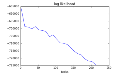
Looking at the above, notice that after a point (150 topics), the number of words chosen levels out.

Topic Words Up & Over a Threshold

This approach chooses words until the cumulative summation is greater than cut off. In this case the desire is to choose 80% of the words in a topic.

Screen Shot 2016-03-25 at 2.41.03 PM

Notice that when there are too few topics far too many words are chosen. One could argue from the above graph, that the optimal bread topics looks to be around or greater than 50.

Of course the above methods are sensitive to the parameters of N, epsilon, or threshold chosen.

Log Likelihood

Screen Shot 2016-03-25 at 2.43.02 PM

Thomas L. Griffiths, Mark Steyvers (2004) suggest to maximize the above graph however it appears to not be satisfactory in this situation.

Normalization

Is it better to not to normalize the prob dist and use the original value in a cut-off?

Looking at another library gensim LdaModel, it appears that LDA most likely does not originally have the probabilities sum up to 1.0 like that and they are normalized, see below:

def show_topic(self, topicid, topn=10):
    topic = self.state.get_lambda()[topicid]
    topic = topic / topic.sum() # normalize to probability dist
    ...

Running the sample code Latent Dirichlet Allocation (LDA) with Python and calling get_lambda, one can see the lambda values are sometimes above 1.0.

ldamodel.state.get_lambda()[1]

gives:

array([ 1.48214337,  1.48168697,  0.50442377,  0.50399559,  0.50400832,
    0.5047193 ,  0.50375875,  0.50376053,  1.50224118,  0.50376574,
    0.5037527 ,  0.50377459,  0.50376621,  1.49831418,  1.49832577,
    1.49831855,  1.49831883,  1.49831596,  1.51053093,  3.49684196,
    1.49832204,  1.49832512,  0.50316907,  0.50321838,  0.50328253,
    0.50319543,  0.50317986,  0.50318815,  0.50314213,  0.5031702 ,
    1.49635267,  1.49634655])

Interestingly the output of Mahout’s cvb local is not normalized to the probability distribution as the gensim library.

{dx4019:53110.68701540677,80048:35567.41624492001,..., dx13629:0.06305282918342679,dxv269:0.05556872163986669}

For the purposes of this study, output from Mahout will be normalized.

Choosing the Word Cut-Off in Claims Analysis

Interestingly, as the number of topics is increased, the initial probability of the top word decreases and levels off to about 8% or so. A possible interpretation of this topics are being split into two but perhaps they should not be. This would suggest that the number of topics may not be higher than 12.

Screen Shot 2016-03-26 at 2.18.14 PM

Using the top eight work method notice that the strength of the top eight words gets diluted as the number of topics increases.

Screen Shot 2016-03-26 at 2.17.14 PM

Using the threshold method the number of codes in the topic levels out after 20 or so.

Screen Shot 2016-03-26 at 2.17.38 PM


When choosing the epsilon method, for determining the number of words, the number of words chosen levels off soon around 15 when epsilon=0.01 and 7 for epsilon=0.02.

Screen Shot 2016-03-26 at 2.20.06 PMScreen Shot 2016-03-26 at 2.17.54 PM

Using the epsilon=0.02 technique and looking at the num_topics=3, one can see that the first topic is largely therapeutic in nature, followed by dialysis and finally the final topic being blood test related.  Oddly, a chest x-ray was included.

eps 0.02
Topic 0
97110 0.13 Therapeutic exercises
80048 0.04 Metabolic panel total ca
99213 0.04 Office/outpatient visit est
97530 0.04 Therapeutic activities
97116 0.03 Gait training therapy
97112 0.03 Neuromuscular reeducation
80053 0.03 Comprehen metabolic panel
97140 0.03 Manual therapy 1/> regions

Topic 1
36415 0.18 Routine venipuncture
q4081 0.12 Epoetin alfa, 100 units esrd
a4657 0.12 Syringe w/wo needle
90999 0.12 Dialysis procedure
j2501 0.07 Paricalcitol
99211 0.03 Office/outpatient visit est
j1756 0.02 Iron sucrose injection
j1270 0.02 Injection, doxercalciferol

Topic 2
85025 0.09 Complete cbc w/auto diff wbc
85610 0.06 Prothrombin time
80053 0.04 Comprehen metabolic panel
80061 0.03 Lipid panel
84443 0.02 Assay thyroid stim hormone
71020 0.02 Chest x-ray 2vw frontal&latl
99212 0.02 Office/outpatient visit est

Going to the other extreme and looking at the data set split into 256 topics, one can notice some topics that appear to be duplicative in nature, however perhaps they are not.  A specialist schooled in the art of dialysis may recognize an important difference.

Topic  6
a4657 0.06 Syringe w/wo needle
q4081 0.05 Epoetin alfa, 100 units esrd
85610 0.04 Prothrombin time
90999 0.03 Dialysis procedure
85025 0.03 Complete cbc w/auto diff wbc
36415 0.03 Routine venipuncture
97110 0.02 Therapeutic exercises
99213 0.02 Office/outpatient visit est
Topic  7
36415 0.09 Routine venipuncture
97110 0.07 Therapeutic exercises
q4081 0.05 Epoetin alfa, 100 units esrd
85025 0.04 Complete cbc w/auto diff wbc
a4657 0.04 Syringe w/wo needle
85610 0.03 Prothrombin time
90999 0.03 Dialysis procedure
Topic  8
90999 0.06 Dialysis procedure
97110 0.05 Therapeutic exercises
a4657 0.05 Syringe w/wo needle
85610 0.05 Prothrombin time
36415 0.03 Routine venipuncture
j2501 0.03 Paricalcitol
q4081 0.02 Epoetin alfa, 100 units esrd
80061 0.02 Lipid panel

The methods utilized in this post maybe sufficient for determining broad categories of care however it appears to not be sufficient to act as a method of determining a catalog procedures.

It is interesting to note, that with the proper choice parameters, one can approximate the frequency of the actual claim lines in the claims.

Screen Shot 2016-03-25 at 1.45.45 PM

Further work in this area may be warranted.

Conclusions

LDA looks effective for discerning the high-level groupings (topics) of procedures but does not do well for this data set for finer more granular groupings.  As for the topic words themselves, using the epsilon approach for topic word selection is superior to the top N words approach while being computationally simpler than the threshold approach. The parameters involved in the epsilon method and the threshold approach can be set to achieve near identical results.   In regards the membership of each word, normalization of the lambda values makes them more interpretable and it is recommended when using Mahout.

Next Steps

As an exercise for the reader, these are the topics with the diagnosis codes included in the word sets. Do these topics look cohesive? Do the topics look disjoint?

eps 0.02

Topic  0
97110 0.14 Therapeutic exercises
97530 0.05 Therapeutic activities
97112 0.04 Neuromuscular reeducation
97140 0.04 Manual therapy 1/> regions
97116 0.03 Gait training therapy

Topic  1
36415 0.07 Routine venipuncture
85025 0.03 Complete cbc w/auto diff wbc
dx4019 0.02 Hypertension NOS
80048 0.02 Metabolic panel total ca

Topic  2
36415 0.08 Routine venipuncture
85025 0.04 Complete cbc w/auto diff wbc
dx4019 0.03 Hypertension NOS
80053 0.02 Comprehen metabolic panel
85610 0.02 Prothrombin time
80048 0.02 Metabolic panel total ca

Topic  3
q4081 0.11 Epoetin alfa, 100 units esrd
a4657 0.08 Syringe w/wo needle
90999 0.05 Dialysis procedure
j2501 0.05 Paricalcitol
j1270 0.02 Injection, doxercalciferol

Topic  4
99213 0.04 Office/outpatient visit est
36415 0.04 Routine venipuncture

Topic  5
97110 0.05 Therapeutic exercises
85025 0.02 Complete cbc w/auto diff wbc
dx4019 0.02 Hypertension NOS
80048 0.02 Metabolic panel total ca

Topic  6
80053 0.05 Comprehen metabolic panel
36415 0.04 Routine venipuncture
85025 0.03 Complete cbc w/auto diff wbc
85610 0.02 Prothrombin time
dx25000 0.02 DMII wo cmp nt st uncntr
80061 0.02 Lipid panel

Topic  7
90999 0.07 Dialysis procedure
a4657 0.07 Syringe w/wo needle
q4081 0.05 Epoetin alfa, 100 units esrd
j2501 0.04 Paricalcitol
36415 0.03 Routine venipuncture
85025 0.03 Complete cbc w/auto diff wbc

A future blog post will examine K-means. That method has a benefit of keeping the topics sets completely separate.

K-Means Claims Analysis

References

Jordan Barber (n.d.) Latent Dirichlet Allocation (LDA) with Python https://rstudio-pubs-static.s3.amazonaws.com/79360_850b2a69980c4488b1db95987a24867a.html

Chris Busch (2016) “Choosing words in a topic, which cut-off for LDA topics?” http://stats.stackexchange.com/questions/199263/choosing-words-in-a-topic-which-cut-off-for-lda-topics

Thomas L. Griffiths, Mark Steyvers (2004) “Finding scientific topics” http://psiexp.ss.uci.edu/research/papers/sciencetopics.pdf

Allen B. Riddell (2014) Topic modeling with latent Dirichlet allocation in Python https://ariddell.org/lda.html

Radim Rehurek (2011) http://pydoc.net/Python/gensim/0.8.6/gensim.models.ldamodel/